MultiAmplicon - a small example • MultiAmplicon

Preparing sequencing read files and a primer set

The MultiAmplicon package uses dedicated classes to ensure that input to its sortAmplicons function is provided correctly. Concerning input files, this means for the user that file names (including paths to the directory they are stored in) of forward and reverse sequencing read files must be provided as a PairedReadFileSet. These files can contain reads in fastq or in gzipped fastq format. We focus as a default use case on (non-interleaved) paired-end reads, as these are the most common format Illumina sequencing reads are currently produced in.

Similarly, primer pairs must be provided in a PrimerPairsSet. We then match forward and reverse primers at the start of forward and reverse reads, respectively. The maximal number of mismatches and the maximal distance from the start of the read can be supplied as arguments to the function. The primer sequences are trimmed from the reads and the read-pair is associated with the amplicon defined by the primer-pair.

We first have a look at how PairedReadFileSet and PrimerPairsSet are generated. Please use files containing quality filtered sequencing reads for the steps below. See the dada2 tutorial or our real-world example vignette for how files are trimmed and quality filtered. But we here first use a very small data set included in the MultiAmplicon package.

library(MultiAmplicon)
## we'll also use some dada2 functions directly
library(dada2)

fastq.dir <- system.file("extdata", "fastq", package = "MultiAmplicon")
fastq.files <- list.files(fastq.dir, full.names=TRUE)

Ffastq.file <- fastq.files[grepl("F_filt", fastq.files)]
Rfastq.file <- fastq.files[grepl("R_filt", fastq.files)]

names(Rfastq.file) <- names(Ffastq.file) <-
    gsub("_F_filt\\.fastq\\.gz", "", basename(Ffastq.file))

PRF <- PairedReadFileSet(Ffastq.file, Rfastq.file)

primerF <- c(Amp1F = "AGAGTTTGATCCTGGCTCAG", Amp2F = "ACTCCTACGGGAGGCAGC",
             Amp3F = "GAATTGACGGAAGGGCACC", Amp4F = "YGGTGRTGCATGGCCGYT",
             Amp5F = "AAAAACCCCGGGGGGTTTTT", Amp6F = "AGAGTTTGATCCTGCCTCAG")

primerR <- c(Amp1R = "CTGCWGCCNCCCGTAGG", Amp2R = "GACTACHVGGGTATCTAATCC",
             Amp3R = "AAGGGCATCACAGACCTGTTAT", Amp4R = "TCCTTCTGCAGGTTCACCTAC",
             Amp5R = "AAAAACCCCGGGGGGTTTTT", Amp6R = "CCTACGGGTGGCAGATGCAG")

PPS <- PrimerPairsSet(primerF, primerR)

MA <- MultiAmplicon(PPS, PRF)

Note that the primer pairs in the PrimerPairsSet can be named and the same also is true for the sequencing read file pairs (although not in our example above). This results in names for primer-pairs and for samples.

Sorting into multiple amplicons

Based on the primer sequences we can now sort the sequences into amplicons. This is done by the function sortAmplicons, which updates the MultiAmplicon object with the sorted amplicons.

For this small example data set we can look at the resulting rawCounts (function getRawCounts) i.e. the number of sequences for each of the fully stratified amplicon x sample matrix.

MA1 <- sortAmplicons(MA, filedir=tempfile("dir"))

knitr::kable(getRawCounts(MA1))

	S01	S02	S03	S04	S05	S05D	S06
Amp1F.Amp1R	0	3495	5	5	29310	29310	2569
Amp2F.Amp2R	0	2949	0	2	20391	20391	2690
Amp3F.Amp3R	0	1817	0	0	0	0	11671
Amp4F.Amp4R	0	1087	0	7	2076	2076	428
Amp5F.Amp5R	0	0	0	0	0	0	0
Amp6F.Amp6R	1	0	0	0	0	0	0

Visualizing read numbers per amplicon and filtering based on these

Now we can plot the result. The function plotAmpliconNumbers allows us also to store clustering information (see ). Which can afterwards be used to filter data.

clusters <- plotAmpliconNumbers(MA1)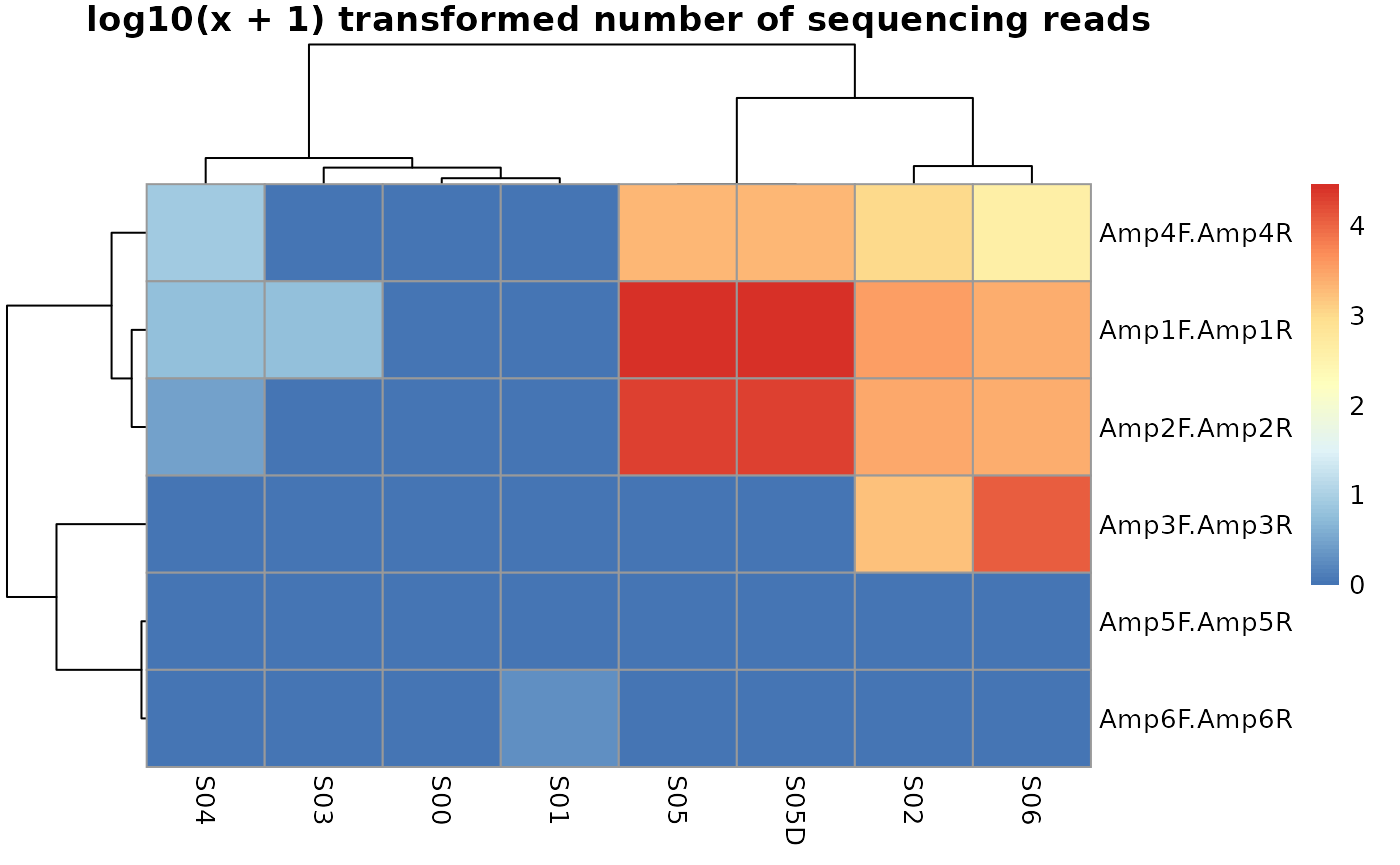

We can use this clustering information now to subset our MultiAmplicon object.

two.clusters.row <- cutree(clusters$tree_row, k=2)
two.clusters.col <- cutree(clusters$tree_col, k=2)

knitr::kable(two.clusters.row)

	x
Amp1F.Amp1R	1
Amp2F.Amp2R	1
Amp3F.Amp3R	2
Amp4F.Amp4R	1
Amp5F.Amp5R	2
Amp6F.Amp6R	2

knitr::kable(two.clusters.col)

	x
S00	1
S01	1
S02	2
S03	1
S04	1
S05	2
S05D	2
S06	2


MA.sub <- MA1[which(two.clusters.row==1), which(two.clusters.col==2)]

knitr::kable(getRawCounts(MA.sub))

	S02	S05	S05D	S06
Amp1F.Amp1R	3495	29310	29310	2569
Amp2F.Amp2R	2949	20391	20391	2690
Amp4F.Amp4R	1087	2076	2076	428

In real world applications (see our other vignette) the samples to be excluded from further analysis can be selected based on clustering with negative controls (similar to the example data here where S00 is an empty file and S01 contains one sequence).

Running the amplicon sequencing pipeline

We first estimate the errors separately for both for dada’s probabilistic sequence variant inference. We do this here on the combined stratified files for different amplicons. This should be done separately for forward ad reverse sequence though!

errF <- learnErrors(unlist(getStratifiedFilesF(MA1)), verbose=0)
errR <- learnErrors(unlist(getStratifiedFilesR(MA1)), verbose=0)

We can now run the pipeline of the dada2 package in parallel over the different amplicons. We update our object from each previous step and safe it under a new name, here for illustration. In your own workflow you can also overwrite the old object.

MA3 <- dadaMulti(MA1, Ferr=errF, Rerr=errR,  pool=FALSE)
#> Sample 1 - 3495 reads in 1493 unique sequences.
#> Sample 2 - 5 reads in 5 unique sequences.
#> Sample 3 - 5 reads in 5 unique sequences.
#> Sample 4 - 29310 reads in 7224 unique sequences.
#> Sample 5 - 29310 reads in 7224 unique sequences.
#> Sample 6 - 2569 reads in 1053 unique sequences.
#> Sample 1 - 3495 reads in 1535 unique sequences.
#> Sample 2 - 5 reads in 5 unique sequences.
#> Sample 3 - 5 reads in 4 unique sequences.
#> Sample 4 - 29310 reads in 8273 unique sequences.
#> Sample 5 - 29310 reads in 8273 unique sequences.
#> Sample 6 - 2569 reads in 994 unique sequences.
#> Sample 1 - 2949 reads in 1142 unique sequences.
#> Sample 2 - 2 reads in 2 unique sequences.
#> Sample 3 - 20391 reads in 4136 unique sequences.
#> Sample 4 - 20391 reads in 4136 unique sequences.
#> Sample 5 - 2690 reads in 968 unique sequences.
#> Sample 1 - 2949 reads in 1290 unique sequences.
#> Sample 2 - 2 reads in 2 unique sequences.
#> Sample 3 - 20391 reads in 5719 unique sequences.
#> Sample 4 - 20391 reads in 5719 unique sequences.
#> Sample 5 - 2690 reads in 1100 unique sequences.
#> Sample 1 - 1817 reads in 589 unique sequences.
#> Sample 2 - 11671 reads in 3783 unique sequences.
#> Sample 1 - 1817 reads in 547 unique sequences.
#> Sample 2 - 11671 reads in 4054 unique sequences.
#> Sample 1 - 1087 reads in 394 unique sequences.
#> Sample 2 - 7 reads in 6 unique sequences.
#> Sample 3 - 2076 reads in 959 unique sequences.
#> Sample 4 - 2076 reads in 959 unique sequences.
#> Sample 5 - 428 reads in 166 unique sequences.
#> Sample 1 - 1087 reads in 433 unique sequences.
#> Sample 2 - 7 reads in 5 unique sequences.
#> Sample 3 - 2076 reads in 962 unique sequences.
#> Sample 4 - 2076 reads in 962 unique sequences.
#> Sample 5 - 428 reads in 183 unique sequences.

MA4 <- mergeMulti(MA3, justConcatenate=TRUE)

MA5 <- makeSequenceTableMulti(MA4)

MA6 <- removeChimeraMulti(MA5, mc.cores=1)

The steps after sortAmplcions until removeChimeraMulti recapitulate different processes in the dada2 pipeline.

A word on dada2 sequence inference

The above workflow assumes that errors could be estimated for each amplicon together. This would be beneficial if errors were largely similar between different amplicons (i.e. not influenced by the primer sequence comprising the first bases the original sequence). Below an alternative approach is demonstrated with error probabilities estimated separately for each amplicon (here we also overwrite objects from each previous processing steps).

MA.alt <- dadaMulti(MA3, selfConsist=TRUE, pool=FALSE)
#> Initializing error rates to maximum possible estimate.
#> selfConsist step 1 ......
#>    selfConsist step 2
#>    selfConsist step 3
#>    selfConsist step 4
#>    selfConsist step 5
#>    selfConsist step 6
#> Convergence after  6  rounds.
#> Initializing error rates to maximum possible estimate.
#> selfConsist step 1 ......
#>    selfConsist step 2
#>    selfConsist step 3
#>    selfConsist step 4
#>    selfConsist step 5
#> Convergence after  5  rounds.
#> Initializing error rates to maximum possible estimate.
#> selfConsist step 1 .....
#>    selfConsist step 2
#>    selfConsist step 3
#>    selfConsist step 4
#>    selfConsist step 5
#>    selfConsist step 6
#> Convergence after  6  rounds.
#> Initializing error rates to maximum possible estimate.
#> selfConsist step 1 .....
#>    selfConsist step 2
#>    selfConsist step 3
#>    selfConsist step 4
#>    selfConsist step 5
#> Convergence after  5  rounds.
#> Initializing error rates to maximum possible estimate.
#> selfConsist step 1 ..
#>    selfConsist step 2
#>    selfConsist step 3
#>    selfConsist step 4
#>    selfConsist step 5
#> Convergence after  5  rounds.
#> Initializing error rates to maximum possible estimate.
#> selfConsist step 1 ..
#>    selfConsist step 2
#>    selfConsist step 3
#>    selfConsist step 4
#>    selfConsist step 5
#> Convergence after  5  rounds.
#> Initializing error rates to maximum possible estimate.
#> selfConsist step 1 .....
#>    selfConsist step 2
#>    selfConsist step 3
#>    selfConsist step 4
#>    selfConsist step 5
#> Convergence after  5  rounds.
#> Initializing error rates to maximum possible estimate.
#> selfConsist step 1 .....
#>    selfConsist step 2
#>    selfConsist step 3
#>    selfConsist step 4
#> Convergence after  4  rounds.

MA.alt <- mergeMulti(MA.alt, justConcatenate=TRUE)

MA.alt <- makeSequenceTableMulti(MA.alt)

MA.alt <- removeChimeraMulti(MA.alt, mc.cores=1)

Now we can make a comparison between the two different versions:

together <- getSequencesFromTable(MA6)
alt <- getSequencesFromTable(MA.alt)

lapply(seq_along(together), function (i){
  union <- union(alt[[i]], together[[i]])
  table("combined Inference"=union%in%together[[i]],
        "seperate amplicon"=union%in%alt[[i]])
})
#> [[1]]
#>                   seperate amplicon
#> combined Inference FALSE TRUE
#>              FALSE     0    6
#>              TRUE      3  219
#> 
#> [[2]]
#>                   seperate amplicon
#> combined Inference FALSE TRUE
#>              FALSE     0   11
#>              TRUE      6  153
#> 
#> [[3]]
#>                   seperate amplicon
#> combined Inference FALSE TRUE
#>              FALSE     0    2
#>              TRUE      1  157
#> 
#> [[4]]
#>                   seperate amplicon
#> combined Inference FALSE TRUE
#>              FALSE     0    2
#>              TRUE      8  116
#> 
#> [[5]]
#> < table of extent 0 x 0 >
#> 
#> [[6]]
#> < table of extent 0 x 0 >

So for all amplicons we got very similar output, the overwhelming majority of ASVs was found using both methods. This speaks for error rates not differing between amplicons (and for the robustness of the ASV inference of the amazing dada2). Which method you should use depends on your data: if each amplicon has enough reads you can estimate seperately and potentially get a better estimate of errors for amplicons with different errors. If on the other hand some amplicons have very few reads, it might make sense to pool them to improve error estimates with larger size for the training set.

Using different parameters for each amplicon

In some real world applications it might be desirable to have more control over parameters used in the pipeline for different amplicons.

We use ellipsis (aka “…”, dots, dot-dot-dot or three-dots) to pass parameters on to the underlying dada2 functions. The MultiAmplicon package allows all those arguments to be vectors with values varying for different amplicons.

Let’s suppose for this we e.g. want to merge a subset of our amplicons, while we concatenate others (with Ns between forward and reverser reads).

MA.mixed <- mergeMulti(MA3, justConcatenate=c(TRUE, FALSE, FALSE, TRUE, FALSE, FALSE))
#> 
#> merging sequences from 6 samples for amplicon Amp1F.Amp1R
#> calling mergePairs with justConcatenate=TRUE parameters
#> 
#> merging sequences from 5 samples for amplicon Amp2F.Amp2R
#> calling mergePairs with justConcatenate=FALSE parameters
#> 
#> merging sequences from 2 samples for amplicon Amp3F.Amp3R
#> calling mergePairs with justConcatenate=FALSE parameters
#> 
#> merging sequences from 5 samples for amplicon Amp4F.Amp4R
#> calling mergePairs with justConcatenate=TRUE parameters
#> 
#> merging sequences from 0 samples for amplicon Amp5F.Amp5R
#> calling mergePairs with justConcatenate=FALSE parameters
#> 
#> merging sequences from 0 samples for amplicon Amp6F.Amp6R
#> calling mergePairs with justConcatenate=FALSE parameters

The above example would make sense if (only) amplicons Amp1F.Amp1R and Amp4F.Amp4R (1st and 4th in our object) had too little overlap between forward and reverse reads to be merged and would better be concatenated. Btw: Here this makes not really sense as to much sequences for the 2nd and 3rd amplicon don’t merge for this dataset.

Coming back to our example on dada sequence inference, we could also mix err estimates to use errors either seperately or accross amplicons. Always set the references to both pre-computed error parameters NULL when using self consistent estimation within one amplicon.

MA.mixed <- dadaMulti(MA3,
                      Ferr=c(NULL, errF,  NULL, errF, NULL, NULL),
                      Rerr=c(NULL, errR,  NULL, errR, NULL, NULL),
               selfConsist=c(TRUE, FALSE, TRUE, FALSE, TRUE, TRUE))
#> 
#> 
#> amplicon Amp1F.Amp1R: dada estimation of sequence variants from 6 of 8 possible sample files
#> calling dada with selfConsist=TRUE parameters
#> selfConsist step 1 ......
#>    selfConsist step 2
#>    selfConsist step 3
#>    selfConsist step 4
#> Convergence after  4  rounds.
#> selfConsist step 1 ......
#>    selfConsist step 2
#>    selfConsist step 3
#>    selfConsist step 4
#> Convergence after  4  rounds.
#> 
#> 
#> amplicon Amp2F.Amp2R: dada estimation of sequence variants from 5 of 8 possible sample files
#> calling dada with selfConsist=FALSE parameters
#> Sample 1 - 2949 reads in 1142 unique sequences.
#> Sample 2 - 2 reads in 2 unique sequences.
#> Sample 3 - 20391 reads in 4136 unique sequences.
#> Sample 4 - 20391 reads in 4136 unique sequences.
#> Sample 5 - 2690 reads in 968 unique sequences.
#> Sample 1 - 2949 reads in 1290 unique sequences.
#> Sample 2 - 2 reads in 2 unique sequences.
#> Sample 3 - 20391 reads in 5719 unique sequences.
#> Sample 4 - 20391 reads in 5719 unique sequences.
#> Sample 5 - 2690 reads in 1100 unique sequences.
#> 
#> 
#> amplicon Amp3F.Amp3R: dada estimation of sequence variants from 2 of 8 possible sample files
#> calling dada with selfConsist=TRUE parameters
#> selfConsist step 1 ..
#>    selfConsist step 2
#>    selfConsist step 3
#>    selfConsist step 4
#> Convergence after  4  rounds.
#> selfConsist step 1 ..
#>    selfConsist step 2
#>    selfConsist step 3
#>    selfConsist step 4
#> Convergence after  4  rounds.
#> 
#> 
#> amplicon Amp4F.Amp4R: dada estimation of sequence variants from 5 of 8 possible sample files
#> calling dada with selfConsist=FALSE parameters
#> Sample 1 - 1087 reads in 394 unique sequences.
#> Sample 2 - 7 reads in 6 unique sequences.
#> Sample 3 - 2076 reads in 959 unique sequences.
#> Sample 4 - 2076 reads in 959 unique sequences.
#> Sample 5 - 428 reads in 166 unique sequences.
#> Sample 1 - 1087 reads in 433 unique sequences.
#> Sample 2 - 7 reads in 5 unique sequences.
#> Sample 3 - 2076 reads in 962 unique sequences.
#> Sample 4 - 2076 reads in 962 unique sequences.
#> Sample 5 - 428 reads in 183 unique sequences.
#> 
#> 
#> amplicon Amp5F.Amp5R: dada estimation of sequence variants from 0 of 8 possible sample files
#> 
#> skipping empty amplicon
#> 
#> 
#> amplicon Amp6F.Amp6R: dada estimation of sequence variants from 0 of 8 possible sample files
#> 
#> skipping empty amplicon

Taxnomic annotation

Taxonimical annotation is difficult as for 18S markers reference databases are not as mature as for 16S. As we use Multiamplicon in our own research it includes for now only a 18S annotation via BLAST+. This only works on UNIX systems with the NCBI BLAST+ toolkit installed. In addition we have to build a taxonomizr database.

## echo=TRUE for this?
inputFasta <- system.file("extdata", "in.fasta", package = "MultiAmplicon")
outputBlast <- system.file("extdata", "out.blt", package = "MultiAmplicon")

MA7 <- blastTaxAnnot(MA6, db="/SAN/db/blastdb/nt/nt",
                     negative_gilist = "/SAN/db/blastdb/uncultured_gilist.txt",
                     taxonSQL="/SAN/db/taxonomy/taxonomizr.sql", num_threads=20,
                     infasta = inputFasta,
                     outblast = outputBlast)
#> file /usr/local/lib/R/site-library/MultiAmplicon/extdata/in.fasta exists, using existing file! To extract input sequences for blast  again delete the file
#> file/usr/local/lib/R/site-library/MultiAmplicon/extdata/out.blt exists, using existing file! To run blast again delete file

In the above code you have to adjust the path’s for the BLAST and taxonomizr databases.

Handing over to phyloseq

The phyloseq package provides impressive tools for microbiome data handling and analysis. We can now convert our MultiAmpicon object into a phlyoseq object. The multi2Single option controls whether we’ll get a single phyloseq object or a list of such objects. In case of a single phyloseq object (multi2Single=TRUE) we get ASVs from diffrent amplicons still as seperate sequences, but all within one object. In case of a a list of phyloseq object (multi2Single=FALSE) we can each of the many phyloseq objects contains only ASVs from one amplicon.

## echo=TRUE for this?
library(phyloseq)

PHY <- toPhyloseq(MA7, samples=colnames(MA7), multi2Single=TRUE)
#> extracting 8 requested samples
#> filling zeros for amplicon missing 3 samples
#> extracting 8 requested samples
#> filling zeros for amplicon missing 4 samples
#> extracting 8 requested samples
#> filling zeros for amplicon missing 6 samples
#> extracting 8 requested samples
#> filling zeros for amplicon missing 4 samples
#> extracting 8 requested samples
#> filling zeros for amplicon missing 8 samples
#> extracting 8 requested samples
#> filling zeros for amplicon missing 8 samples
PHY.list <- toPhyloseq(MA7, samples=colnames(MA7), multi2Single=FALSE)
#> extracting 8 requested samples
#> filling zeros for amplicon missing 3 samples
#> extracting 8 requested samples
#> filling zeros for amplicon missing 4 samples
#> extracting 8 requested samples
#> filling zeros for amplicon missing 6 samples
#> extracting 8 requested samples
#> filling zeros for amplicon missing 4 samples
PHYgenus <- tax_glom(PHY, "genus")

knitr::kable(table(tax_table(PHYgenus)[, "superkingdom"]))

Var1	Freq
Bacteria	19
Eukaryota	30

knitr::kable(table(tax_table(PHYgenus)[, "phylum"]))

Var1	Freq
Actinobacteria	1
Apicomplexa	4
Ascomycota	4
Basidiomycota	6
Cercozoa	1
Chlorophyta	4
Ciliophora	1
Endomyxa	2
Evosea	1
Firmicutes	14
Fusobacteria	2
Mucoromycota	1
Nematoda	2
Platyhelminthes	1
Proteobacteria	2
Streptophyta	2

MultiAmplicon - a small example

Emanuel Heitlinger

2021-01-20